Snakes and Lagrangian Ladders.
Published 29 December 2024 at Yours, Kewbish. 4,779 words. Subscribe via RSS.
Introduction
I recently had the pleasure of reading a dense crypto paper, emailing the corresponding author in frustration to ask questions, then double emailing two hours later to say I’d figured it out. The paper in question was Yurek et al.’s “Long Live The Honey Badger: Robust Asynchronous DPSS and its Applications”: it describes how to split up a secret into shares that can be distributed among a set of people and how to change the set of people and refresh shares while keeping the original secret intact. Secret sharing is important for sensitive but critical information: information that no single party should be able to read on their own, but that we can’t afford to lose — think nuclear launch codes and encryption keys.
The problem I was emailing with was me not being able to understand the refresh process. Algorithm 3 in the paper opaquely says a few times to “interpolate” the desired new secrets. I’m sure seasoned cryptographers can recalculate secrets from shares in their sleep, but detangling these three lines took more time than reading the entire rest of the paper. Typical secret sharing via Shamir secret sharing is very cleverly constructed already, and as I mentioned in my previous post, crypto papers generally don’t do a good job of explaining the basics in favour of just laying down novel material. This is great for brevity and conciseness in academia, but not so great for beginners to the field.
Once I’d gotten more background on the very finicky math, the actual interpolation and refreshing wasn’t hard to understand and implement. Still, I wish they’d linked to a layman’s explainer, although from a few cursory searches, none quite seems to exist. This post is the explainer I wish I’d had before tackling this paper. I’ll cover the very basics of Shamir secret sharing before summarizing the Honey Badger protocol’s use of interpolation, explaining the key three lines of Algorithm 3 in the scheme, so you can hopefully save yourself the three hours of puzzling.
Eating the Frog
In my opinion, the hardest part of Shamir Secret Sharing is the Lagrange interpolation, so I’m going to put it up front here while your brains are still fresh. Lagrange interpolation is a way of estimating the value of a polynomial at some input, given some points on the polynomial. Let’s consider a bog-standard function: f(x) = x^2 + 2.

Figure 1. f(x) = x² + 2
If we have no knowledge of the polynomial, we’ll need three points to estimate the value of f(x) for any x back. This is because f(x) is a polynomial of degree two (highest power term is x^2). There’s no x term in the function as I’ve written it, but we can also write it as f(x) = 1 * x^2 + 0 * x + 2.
In order to recover f(x), we need to solve for the coefficients of the terms — the 1, 0, and 2. If we know the values y_i = f(x_i) taken at few different points x_i, then we’ll get something like the below:
y_1 = a * x_1^2 + b * x_1 + c
y_2 = a * x_2^2 + b * x_2 + c
y_3 = a * x_3^2 + b * x_3 + c
In this case, we know three values of x, and their associated y values, and we’re solving for a, b, and c. Because we have three unknown coefficients, we’ll need a system of three equations, based on three evaluated points. In general, for a polynomial of degree t, you’ll need t+1 points to solve for the polynomial — the extra +1 comes from the unknown value of the constant term itself.
To figure out how to reconstruct the polynomial, let’s start with a slightly easier function, f(x) = 2x. Let’s say we know that f(1) = 2 and f(3) = 6.
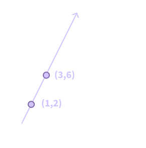
Figure 2. f(x) = 2x
We want to derive a polynomial that takes on the value 2 at x = 1 and 6 at x = 3. This is one such polynomial:
y = (x - 3)/(1 - 3) * 2 + (x - 1)/(3 - 1) * 6
Note that when x = 1, the first fraction cancels out to 1 and the second fraction evaluates to 0, so y = 1 * 2 + 0 * 6 = 2, as expected. Similarly, when x = 3, the first fraction evaluates to 0 and the second fraction to 1, making y = 0 * 2 + 1 * 6 = 6. Also note that when we rearrange the terms:
y = (x - 3)/(-2) * 2 + (x - 1)/(2) * 6
  = -(x - 3) + 3(x - 1)
  = -x + 3 + 3x - 3
  = 2x
So we can recover our original function! As another example, let’s take our original function f(x) = x^2 + 2. Because this polynomial is of degree 2, we’ll need 3 points to reconstruct it. Let’s take f(1) = 3, f(2) = 6, and f(3) = 11.
Let’s look at the form of our fractional coefficients. We want each fraction to evaluate to 1 at the associated x-value, so the overall term evaluates to the right y-value. We also want the fraction to evaluate to 0 anywhere else. The general form of such a term (let’s say, for the point (x_i, y_i)) is to have the numerator of the fraction be a product of (x - x_m), and the denominator be (x_i - x_n), for all of the other x_m. We exclude the (x - x_i)/(x_i - x_i) fraction, because when this is evaluated at x_i, we’d get 0/0, which is undefined. When we evaluate this fraction at x_i, the terms in the numerator all cancel with the terms in the denominator, so we get 1, as desired. When we evaluate this fraction at any of the other input x-values, however, one of the numerator terms (x - x_m) will be 0, preventing this particular y-value from affecting the overall polynomial’s value. This fractional coefficient is also called the Lagrange basis polynomial, and we’ll denote it λ_i(x). Each y-value is multiplied by a different Lagrange basis polynomial, since the x-value changes, so the i in the basis polynomial also has to change.
Figure 3. Form of the Lagrange basis polynomial.
For our example, our polynomial is thus:
y = (x - 2)(x - 3)/(1 - 2)(1 - 3) * 3 +
    (x - 1)(x - 3)/(2 - 1)(2 - 3) * 6 +
	(x - 1)(x - 2)/(3 - 1)(3 - 2) * 11
If we plug in x = 4, for example, we’d expect to get 4^2 + 2 = 18. Indeed, we get:
y = (4 - 2)(4 - 3)/(1 - 2)(1 - 3) * 3 +
    (4 - 1)(4 - 3)/(2 - 1)(2 - 3) * 6 +
	(4 - 1)(4 - 2)/(3 - 1)(3 - 2) * 11
  = 1 * 3 - 3 * 6 + 3 * 11
  = 3 - 18 + 33 = 18
Feel free to skip this expansion, but if you’re interested, this is what we get when we rearrange the terms:
y = (x^2 - 5x + 6) * 3/2 +
    (x^2 - 4x + 3) * -6 +
    (x^2 - 3x + 2) * 11/2
  = (3/2 - 6 + 11/2) * x^2 +
    (-15/2 x + 24 x + - 33/2 x) +
	(9 - 18 + 11)
  = x^2 + 0x + 2 = x^2 + 2
Even when evaluating this interpolated polynomial at an x-value that wasn’t originally provided, like x = 4, for example, we were still able to get the correct result. We can use the same interpolated polynomial to evaluate the y-value at x = 2.5, for example. Using the Lagrange interpolation to recover the y-value at an x-value not included in the list of input points is critical to how Shamir secret sharing works, as I’ll describe in the next section.
Here There Be Snakes (SSS)
Shamir Secret Sharing starts with the secret s that you want to be able to reconstruct. This might be something like a recovery key or private message. For the sake of explanation, assume this secret is a number. In more realistic scenarios, the secret is likely some series of bytes which need to be transcoded into, or at least interpreted as, large integers, but this is outside of the scope of the SSS algorithm.
We then define a polynomial SSS(x) = s + a * x + b * x^2 + ... + z * x^t. The degree of the polynomial (the choice of t) determines how many shares you’ll need to reconstruct the secret s. The coefficients a, b, ... are all randomly chosen numbers. Note that the constant term is the secret s that we’re trying to split into shares, and that SSS(0) = s. The SSS shares of the secret are now simply the point (i, SSS(i)) for some index i — we need to keep track of the actual index from which a SSS share was calculated for the reconstruction later on. Many such shares can then be calculated and distributed to the other parties who want to be able to help reconstruct the secret.
To recover the secret, at least t+1 parties must submit their shares. Using Lagrange interpolation, we can then recover the original SSS polynomial, or in particular, evaluate it at index 0. This gives us the value of s back.
As you might have guessed, SSS’s primary application is data recovery. For example, PreVeil is an E2EE platform focusing on email and file collaboration. It supports the notion of Approval Groups, a recovery scheme that makes use of SSS, requiring some threshold of designated contacts to recover the user’s encryption key. Trezor, the hardware cryptocurrency wallet, makes use of SSS to back up the user’s recovery key. The HN- and GitHub-famous Horcrux tool is one of my favourite SSS applications, just because it’s such a fun concept: Horcrux lets you split up a file into encrypted shares, much like Voldemort did with his soul. I mentioned above that the SSS secret is usually some series of bytes interpreted as a large integer — here, Horcrux splits up the file into chunks of bytes to avoid integer overflow and repeats the SSS once per chunk, collecting the i-th shares of each chunk into the overall i-th share.
With SSS, you can choose both your recovery threshold, t, and your total number of shares, n. Having a large n is appealing, since you have more options for who can help reconstruct your secret — in the case where you’re trying to recover a key from unreliable P2P nodes, for example, the higher availability from a large n might be desirable. On the other hand, an adversary also has more options for who to compromise in order to learn s. Having n be much larger than t can be problematic in this case.
One key caveat of SSS is that when these applications directly recover data (e.g. split up a recovery key directly into shares), they’re vulnerable to malicious parties colluding to recover your data. SSS is usually applied in E2EE contexts as an alternative to the platform servers storing the user’s key, so it’s problematic if adversaries can compromise a threshold of nodes and directly recover your key. In the case when these parties are social recovery contacts (read: real people), social engineering is also a risk, since there’s no easy way to authenticate reconstruction requests, so your contacts might accidentally send their share to a malicious impersonator and leak your recovery data. PreVeil’s whitepaper doesn’t mention any protections against this, and neither does Trezor. I think the collusion and social engineering concerns are fundamental to vanilla SSS without any additional security considerations.
One solution to these issues is the approach I took in my recent research project, Kintsugi, which involves adding an Oblivious Pseudo-Random Function exchange that protects against the risk of collusion by requiring an additional brute-force step, and against social engineering by not requiring recovery request authentication. The math is quite neat, and this project is what made me look at dynamic proactive secret sharing in the first place. Speaking of, let’s get into the Honey Badger protocol now that we have the background on the base SSS protocol.
(Re)sharing is Caring
Honey Badger is the dynamic, proactive secret sharing (DPSS) protocol proposed by Yurek et al. in their 2022 paper “Long Live The Honey Badger: Robust Asynchronous DPSS and its Applications”. DPSS is used to refresh the secret shares that SSS outputs while keeping the same overall secret s. DPSS both allows users to update the set of parties that possess shares, and invalidates former secret shares, preventing them from being used to reconstruct the secret s.
Recall that the SSS polynomial has the form SSS(x) = s + a * x + b * x^2 + ... + z * x^t. I’ll use the term “party” to refer to the party that holds a secret share, be that a service provider, server, or friend. The core idea of Honey Badger is for each party at index i that has the old SSS secret share s_i = SSS(i) to generate a new SSS polynomial:
SSS'_i(x) = s_i + a' * x + b' * x^2 ... + z' * x^t'
The constant term of this new polynomial is the former SSS secret share. The coefficients a', b', ... z' are new random coefficients, and the degree of the polynomial can change to a new threshold t'. The new secret share that results from the DPSS process will be different than s_i, and if they differ, a threshold of t' will be required to reconstruct s instead of a threshold of t. (The Honey Badger paper uses the notation χ_i(x) instead of SSS'_i(x), [s]^i_d instead of s_i, and d instead of t.)
The party at index i then sends an evaluation to each other party at their respective index, SSS'_i(j). which allows the party at index j to interpolate their new share s_j' (line 208 in Algorithm 3 of the paper). These new party shares can be further interpolated to recover the original secret s. Recall that each original s_i = SSS(i) and s = s_0 = SSS(0). Similarly, each party’s new share s'_i is interpolated as SSS'_0(i), or alternative shares of s_0 = s. Once the party at index i has collected a threshold of shares of the form SSS'_1(i), SSS'_2(i) and so on, they can interpolate :
s'_i = λ_1(0) * SSS'_1(i) + λ_2(0) * SSS'_2(i) + ... + λ_{t'}(0) * SSS'_{t'}(i)
    = SSS'_0(i)
Thus, when these s'_i are interpolated again (during a normal SSS recovery operation, for example), the original s is recovered.
  λ_1(0) * s'_1 + λ_2(0) * s'_2 + ... + λ_{t'}(0) * s'_{t'}
= λ_1(0) * SSS'_0(1) + λ_2(0) * SSS'_0(2) + ... + λ_{t'}(0) * SSS'_0(t')
= SSS'_0(0)
= s_0 = s
Intuitively, consider that the original secret s is split into shares once, with each of those party shares being split up again. This broadcast changes which parties hold which sub-shares of the original secret, although the underlying shared data remains the same. SSS'_i(x) can have a different degree, and therefore a different reconstruction threshold t', than SSS(x), allowing users to add or remove recovery parties. This secret refresh can also be configured to run at some desired interval (e.g. once per day) to protect against recovery parties’ shares being leaked over time.
Alternatively, the paper describes this interpolation process more formally by framing the new SSS'_i(x) as a bivariate polynomial, or a polynomial with two variables, denoted as SSS'(i, x) (the paper uses B(x, y), see line 207 of Algorithm 3 in the paper). This bivariate polynomial still has the form SSS'(i, x) = s_i + a' * x + b' * x^2 ... + z' * x^t'. Note that SSS'(0, 0) = s_0 = s. The idea of resharing is then to interpolate in one variable first, i, over the evaluations at x = i (this is the tricky part!) to get the various SSS'(0, i) = s'_i shares. Then, to reconstruct the original secret, you can interpolate in the other variable, x, to recover SSS'(0, 0) = s. If looking at concrete code makes this easier to understand, feel free to also take a look at my Rust implementation and its tests.
Commitment Issues
The above section focused on how the core resharing of Honey Badger worked. However, you might have noticed that the actual paper also mentions checking commitments. Commitments hide an actual value and later prove, upon revealing the value, that you haven’t changed it in the meantime. In Honey Badger, the commitments serve to prove that the nodes are resharing correct secret shares s'_i to the new set of parties.
Honey Badger uses Pedersen commitments, of the form s_i * G + ŝ_i * H (see my other post if you’re less familiar with elliptic curves.) Here, s_i is the secret you’re committing to, G is the generator point of the elliptic curve, ŝ_i is a random blinding factor used to keep s_i secret even in the case of brute-force attacks, and H is similarly a random elliptic curve point. Points G and H are public to both the old and new resharing parties. During refresh operations, ŝ_i is also calculated the same way s_i is reshared, with a new SSS'_i(x) polynomial with ŝ_i as its secret constant.
In Honey Badger, parties broadcast their new shares alongside a new commitment, which is then verified at various points (lines 205 of Algorithm 1, 303 of Algorithm 2, and 202 of Algorithm 3). Nodes must also keep track of other parties’ commitments, though, so they have something to verify new shares against: note that in Algorithm 1, the commitments of all shares are broadcast and stored by all parties. This means that the resharing process requires an additional step to interpolate the new commitments (line 209 of Algorithm 3). This isn’t trivial (in contrast to the paper’s rather flip suggestion to simply ‘interpolate’), because we don’t know the other parties’ new secret shares s'_i or their blinding factors ŝ'_i, so we need to somehow interpolate their new commitments only based on public information.
Let’s say that the party j wants to interpolate these new commitments. To set the scene, we start out by knowing c_i = s_i * G + ŝ_i * H for all of the other parties (without knowing their s_i or ŝ_i, or any of the new shares or blinding factors), as well as our new share s'_j and new blinding factor ŝ'_j. We want to figure out c'_i = s'_i * G + ŝ'_i * H.
The key here is to recall how s'_i is calculated with Lagrange interpolation, which we can also apply on the commitments themselves to interpolate the new c'_i. Recall that the Lagrange basis polynomial, λ_i(x_i), is used as a coefficient for the point at index i to interpolate for the value of the polynomial at x = x_i. Now, instead of interpolating for s_0 at x = 0, we want to interpolate for the commitment at index i. This can be written as:
λ_1(i) * c_1 + λ_2(i) * c_2 + ... + λ_{t+1}(i) * c_{t+1}
We can then expand the form of the commitments c_1, c_2, etc.:
= λ_1(i)     * (s_1 * G     + ŝ_1 * H) +
  λ_2(i)     * (s_2 * G     + ŝ_2 * H) + ...
  λ_{t+1}(i) * (s_{t+1} * G + ŝ_{t+1} * H)
Then, multiply out the Lagrange basis polynomials and collect like terms to move G and H outside. You can then notice that the coefficients of G and H are then exactly the forms of the reshared s'_i and ŝ'_i1.
= (λ_1(i) * s_1 * G + λ_2(i) * s_2 * G + ... + λ_{t+1} * s_{t+1} * G) +
  (λ_1(i) * ŝ_1 * H + λ_2(i) * ŝ_2 * H + ... + λ_{t+1} * ŝ_{t+1} * H)
= (λ_1(i) * s_1 + λ_2(i) * s_2 + ... + λ_{t+1} * s_{t+1}) * G +
  (λ_1(i) * ŝ_1 + λ_2(i) * ŝ_2 + ... + λ_{t+1} * ŝ_{t+1}) * H
= s'_i * G + ŝ'_i * H
= c'_i
This lets us determine the value of c'_i from the other received commitments without actually needing to learn the secret shares of other parties. You can see this commitment interpolation in code here, with tests here.
I’ll admit I couldn’t have figured out how to interpolate these commitments without leaning on ChatGPT — I was barely familiar with single-variable Lagrange interpolation and couldn’t fathom how I could manage both the secret sharing and the blinding factor. This term was the first where I bothered to try using it as a learning tool, and I was pleasantly surprised by how decent it was for crypto in particular. Sometimes, it’d get the explanation itself wrong, but while walking through it, I’d manage to get a key insight that let me fill in the rest correctly. Its errors were fairly easy to spot, especially when translating its output into code: things like mixing up scalar and point addition that an additional reprompt was often enough to fix.
Conclusion
I hope this explainer has highlighted that the crypto isn’t as scary as it sounds, and that the primitives of a paper aren’t so hard to understand either. I think it’d be neat if we required authors to submit a “from the basics” guide alongside their work, even if just to call out what commonly-understood terms like “interpolate” mean and where to look for further information2.
This isn’t intended at all as a dig to the paper, which was otherwise very thorough and well-written. It was easy to read, and I appreciated the various comparison tables and practical benchmarking sections. The paper was a fundamental building block to my recent research work, and I’d definitely recommend giving it a read. There’s plenty more aspects of the paper that I haven’t covered here, including how high-threshold secret sharing is handled and how they optimize resharing by amortizing batched operations. I wanted to focus this blog post on the main interpolation mechanisms in Algorithm 3, but here’s a few more less-fleshed-out notes about Honey Badger:
More pointers on Honey Badger's properties
In the resharing section, we learned how we can recover the original secret s, but we still need to distribute the shares to the various parties. The paper outlines two options: one is to assume the presence of some trusted dealer, with full (albeit perhaps temporary) knowledge of the secret, and the other is to use a distributed key generation function (DKG), which can be used for a trustless setup. If we want to go the DKG route, however, the hitch is that Honey Badger is asynchronous, meaning that it’ll continue to operate in face of arbitrary network delays. This therefore means that the DKG we choose also needs to be asynchronous. This is tricky, since you’d usually expect DKGs to require some element of synchronization and consensus over which nodes to ’listen to’ during key generation. Honey Badger calls out Das et al.’s asynchronous DKG in particular — if you’re interested in detangling this, I’d recommend watching their conference presentation for the same paper first.
Besides asynchrony guarantees, Honey Badger is also Byzantine-fault tolerant up to a third of nodes. This means that even if up to a third of nodes go rogue and actively try to submit incorrect shares for resharing or otherwise misbehave, Honey Badger can still continue with its resharing and refreshing operations. This is thanks to the multi-valued validated Byzantine agreement (MVBA) protocols used to agree on which nodes have emitted correct shares. I’ll discuss this more in the next section on polynomial commitments. You can find their example implementations here — I didn’t fully get my MVBA prototype working in time.
One last note I’ll make is a distinction between the types of failures that Honey Badger can tolerate. One failure, as I’ve just mentioned, is a Byzantine-fault failure, with actively malicious nodes. Honey Badger can handle up to a third of total nodes being Byzantine. On the other hand, it can only tolerate t honest-but-curious nodes that follow the protocol correctly (e.g. don’t submit false s_i) but collude. Any more, and they’ll be able to reconstruct s due to how SSS works. Otherwise, the SSS can instead tolerate having n - t - 1 nodes being offline, since only t+1 nodes are required to successfully recover s. I ran into these differences while trying to describe the overall fault-tolerance of a protocol I was developing that made use of Honey Badger, so I think it’s worth considering here.
If you’re interested in other types of secret sharing, there are so, so many extra offshoots built off the same primitives that you can explore:
- Proactive secret sharing, as mentioned above, is secret sharing where the shares are refreshed while keeping the secret itself the same. Here’s one of the seminal papers on this topic.
- Dynamic secret sharing, as mentioned above, lets the set of parties holding shares to change. Usually, this requires proactive secret sharing — otherwise, former shareholders could collude to reconstruct the secret. This is sometimes also called mobile secret sharing. Here’s another paper on this.
- Computationally secure secret sharing limits the computational resources required to store shares. Secret sharing can require a lot of storage — growing linearly in the number of shares created. This approach allows for more efficient sharing.
- Similarly, batched secret sharing makes sharing multiple secrets more space-efficient. The Honey Badger paper includes a batch-amortized variant, and here’s another paper on the topic.
- Verifiable secret sharing allows parties to validate the correctness of a share. Here’s one paper on this.
- Threshold signatures are slightly different than threshold secret sharing, but there are interesting papers on this as well.
I’m sure there are plenty more variants I’ve missed above — it became a bit of a game during my initial literature review to figure out which magic keyword combination I needed to find relevant papers.
In other news, my workshop paper on decentralized E2EE key recovery was accepted! It builds on the concepts I’ve mentioned in this post and my previous one on OPAQUE. The project is called Kintsugi, a play on how the protocol mends together encryption key backups from distributed shares. The demo implementation is on GitHub, and I’ll update with a copy of the paper when that’s available. I’m pretty proud of the fact I was able to go from knowing very little about cryptography to defining an interesting research direction to implementing and writing a whole paper in less than ten weeks. I’m happy that the project had a solid implementation portion and a focus on applied work, since historically I haven’t sat well with theory-only projects. Nonetheless, I appreciated the stretch to dive into the technical bits of cryptography, as opposed to glossing over it and reaching for existing libraries. There’s still plenty of design considerations to be finalized and details to be polished on the demo, which I’ll be working through next, but this project has been an extremely fun and challenging exercise in cryptography and protocol design.
There are still a few papers that I’ve waded through and think could be explained much better, so I might make this type of cryptography/systems paper explanation a running series here. Wrestling with papers more deeply more often has been a goal of mine for a while, and distilling it into explainers à la Murat is helpful for keeping you accountable for carefully reading all the details. I have my eye on a few systems implementations papers, or perhaps a more theoretical look at a distributed key generation protocol, so we’ll see what I come up with.
-
The keen-eyed reader might notice that we’ve been mixing scalar and point addition for the interpolation process. This has been termed doing the interpolation ‘in the exponent’ — although the elliptic curve notation used here implies group multiplication, the result is equivalent to as if we’d done the commitment interpolation in field arithmetic via exponentiation, then multiplied by the appropriate points. ↩︎
-
It’s occurring to me that this might just be what appendices are commonly used for, but ideally this explainer should be in more casual language! We don’t need thirty pages of proofs and all these Greek symbols to understand how to connect the dots to find a polynomial. ↩︎